Anisotropy is noted when there is a difference measured depending upon the direction something is measured. A common example would be from wood grain. A square piece of pine board will easily break along the lines of the grain but is much more difficult to break against the grain. This difference can be measured in the amount of force needed to break the board.
In the example of the Michelson-Morley experiment, anisotropic difference was the expected result if the aether were present and if the speed of light were variable. The “null result” reported from the experiment was that no anisotropic difference was obtained in the experiment.
The purpose of the rotation of the instrument during the experiment was to look for anisotropic difference based upon the position of the Lecher line. If the speed of light is constant, and if there is no change in the input of the Lecher line, then there can be no cause for a change in the electrical output of the Lecher line. It is the change in the measured output from the assigned location, after rotation of the instrument, that clearly demonstrates the anisotropic difference. It is this difference that has been measured by this experiment that makes the results so important to the current understanding of physics.
The probe setting you select will affect the measured output of the lecher line. However, it will not affect if the result provides an anisotropic difference. Early experimentation was completed without using any probe (the electrical outlet was run from the assigned location on the lecher line with insulated wires that were connected to a BNC adapter) and with a probe setting of x1. The results demonstrated an anisotropic difference, but the results were far greater than the predicted results. Via discussions with the manufacturer of the oscilloscope, it was recommended that x10 setting with the probe would be most appropriate for the 17 MHz frequency that was being transmitted. This setting allowed for a more accurate measurement of the output.
It should be noted that the oscilloscope used with this experiment has multiple settings that can be adjusted including the sample rate, probe setting, and it even has a band pass filter setting among the many others. Changing the settings will frequently change the output measurement. However, changing the output measurement does not change the presence of the anisotropic difference.
It should be further noted that the smaller the output voltage measured from the Lecher line by the oscilloscope, the smaller the anisotropic difference will be. As such I work to find the setting and location on the lecher line that provides the greatest electrical output measurement from the Lecher line. Finally, be aware that if your anisotropic difference is smaller than what can be measured by your effective bit resolution, then your results will not show an anisotropic difference. With this equipment, I have worked to have an output from the Lecher line that will provide no less than a 4 mV difference. If your experiment is near the edge of your equipment’s capabilities, measuring the Vrms, as opposed to the peak voltage, may provide you with a small amount of greater sensitivity. This is due to the math associated with the Vrms measurement.
If you are attempting to replicate the experiment using the 17 MHz frequency, then use a standard oscilloscope probe that has been calibrated via the manufacturer’s recommendations. Then the probe setting on the probe should be x10 and the setting on the oscilloscope should also be x10.
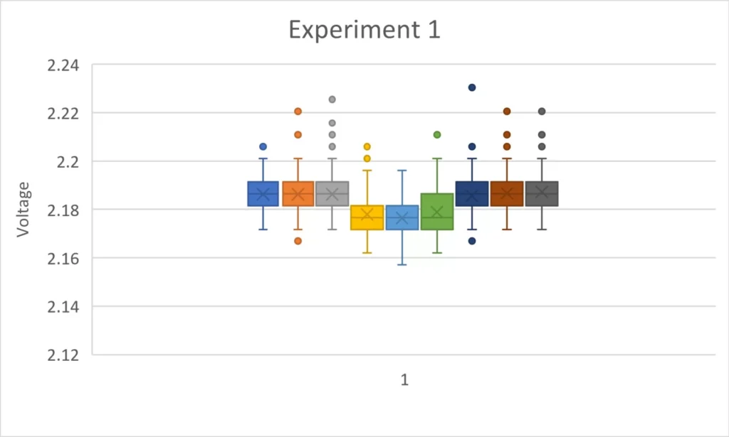
The results obtained in this experiment have a certain amount of variation that is obtained with every experiment. Many causes may be related to this variation, however since it has not affected the ability to demonstrate obvious anisotropic difference, I have not worked to limit the variation beyond what has been needed to complete this experiment. Instrumentation with greater resolution and additional filtering may provide a greater measurement of the output. However, since the exact output is rarely exactly the same, the graphic representation needs to be able to easily demonstrate any difference.
Charting the output as a line graph has been helpful in early experiments and the line graphs will easily demonstrate the anisotropic difference, however when the difference is small, the line graphs tend to run over each other and are less helpful than the box and whisker plot that is provided with the results. It should be noted that line graphs can be useful in seeing causes of problems with data obtained. Thermal variation will present as a gradual increase or decrease in the results over time. Issues with radio frequency interference frequently presents as a hump on the graph and may occur at regular intervals.
The raw data for each experiment is available on this site to download and you can review the data using any graph or data software you choose.
The raw data is available on this website. It is stored in a google drive and linked to the results displayed here. Go to the results section of this website, choose an experiment, and when the page for that experiment is displayed, you will find a link to view the raw data obtained.
I have provided experimental results from a wide variety of situations using various frequencies, voltage inputs, assigned locations, different probe and oscilloscope settings and even different instruments. If the results I provided were from only one instrument with the exact same settings every time, then the results would be more similar in the results. However, a simple change in the daily temperature of the laboratory can cause very small
For this experiment, I have documented the oscilloscope setting “Bit resolution.” The oscilloscope utilized in this experiment provides a setting of “8 Bit” resolution and “16 Bit” resolution. However, selecting “16 Bit” does not actually provide 16 bits of resolution from the oscilloscope. Choosing “16 Bit” allows the oscilloscope to adjust the resolution based upon the sampling frequency (rate) of the oscilloscope. A lower sampling frequency allows for a higher resolution. It should be noted that the sampling frequency should be at least twice the transmitted frequency of from the signal generator to comply with the Nyquist theorem regarding such measurements. In the experiments where effective bit resolution is provided, it is determined using a chart from the oscilloscope manufacturer that lists the effective resolution based upon the sampling rate. This chart is provided below.
| ADC Bit Resolution | 10 Bits (can be reduced to 8 bits) | |||
| Enhanced ADC Bit Resolution (available only when Sampling Frequency is less than 100 MHz) | 16 Bits If this option is selected, the effective bit resolution increases from 10 bits to up to 16 bits as the sampling frequency goes down. (Assuming white noise in the signal) | |||
| Sampling Frequency | Effective Bit Resolution | Sampling Frequency | Effective Bit Resolution | |
| ≥ 100 MHz | 10 Bits | ≤ 25 MHz | 11 Bits | |
| ≤ 6.25 MHz | 12 Bits | ≤ 1.563 MHz | 13 Bits | |
| ≤ 391 kHz | 14 Bits | ≤ 97.7 kHz | 15 Bits | |
| ≤ 24.4 kHz | 16 Bits | ≤ 6.10 kHz | 16 Bits | |
| ≤ 1.526 kHz | 16 Bits | |||
The Nyquist theorem describes sampling rates for pure sine waves. In the simplest terms, it suggests that to accurately measure results from a digitized sine wave, the sampling frequency must be at least twice the frequency of the signal being measured. For more detail, see https://www.techtarget.com/whatis/definition/Nyquist-Theorem
Effective bit resolution can be seen as the microscope from which you are looking at the signal obtained in the experiment. If you don’t have the resolution to observe the anisotropic difference, it will be as if there is no difference at all. As such, you must be able to obtain the measurement from the assigned location at the Lecher line and then predict the anisotropic difference. If the predicted difference is smaller than the minimum resolution you can obtain with your instrumentation, then no difference will be observed. A chart is provided below to demonstrate the minimum anisotropic difference observable based upon the effective bit resolution.
| Effective Bit Resolution | Smallest Observable Anisotropic Difference |
| 8 Bit | 3.92 mV |
| 10 Bit | 0.98 mV |
| 12 Bit | 0.244 mV |
| 14 Bit | 61 µV |
| 16 Bit | 15 µV |
The frequency used for this experiment was a compromise based upon the signal generator I was using and the oscilloscope. It was also based upon the length of the antenna and my ability to rotate the antenna in the lab.
A lower frequency signal would result in a greater wavelength. As the wavelength increases, the output on the Lecher line decreases. As such, the output at the assigned location was so small that the change expected was unlikely to observed by the resolution available. However, at the settings utilized for this experiment, the resolution was adequate to observe an anisotropic difference without needing higher resolution.
The mathematics for predicting the anisotropic difference are described in the paper related to his experiment. For simplicity in the FAQ, simply obtain a voltage output measurement from the assigned location of the lecher line. Then take that measurement and multiply it by 1.00021047. Subtract result of this multiplication from the original output measurement. The final result is an absolute value of the anisotropic difference that is predicted. This predicted value should be the value used when determining if your settings are likely to provide the effective bit resolution for observing the anisotropic difference.
I want to reiterate that while this prediction has been the foundation for which I have set my instrumentation to ensure I can observe the result, my results have been greater than predicted. Since probe settings and other settings can affect the measurement demonstrated on oscilloscope, your results may also be higher than expected. However, when experimenting with settings where the bit resolution was at the edge of what was predicted, results obtained showed much smaller changes and were difficult to see. Whenever possible, use settings that provide you with the greatest possible predicted changes.
This technological advance will most certainly lead to new inventions. As the foundations of physics adapt to these new findings, improvements in computer technology, cosmology and energy are likely to advance in a logarithmic fashion. Currently, these recent findings have set the foundation for a “speedometer” that can be used by spacecraft traveling at near the speed of light.
The results from this experiment have also demonstrated that the Lecher line can be used for gravitational wave detection. NASA is currently working on developing a gravitational wave detector to be placed in space using an interferometer via multiple satellites. This project could be completed via a CubeSat and a lecher line at a fraction of the cost of current plan and without such a technologically challenging plan.
Additionally, results suggest that this technology can possibly be utilized in the fusion process to increase the output of a fusion reactor.
This is the question that will challenge scientists for years. Numerous physicists have written in multiple peer-reviewed journals about the results obtained from the Michelson-Morely experiment and have mathematically challenged the null result. Many others have written papers describing the possibility of variable speed light (VSL) theory without providing any new experimentation to support such theory. This experiment is the experiment that now supports VSL theory.
Both of these experiments are looking for a phase change in the transmitted signal that occurs with movement of the instrument to observe anisotropy. Technologically, measuring the phase change of a 17 MHz signal from a Lecher line is much less difficult than measuring a phase change of a light wave at the incredibly small wavelength that is produced during the experiment.
Most scientists have never built an interferometer with the capability and sensitivity to accurately measure an anisotropic difference. It’s technically difficulty and expensive to do such an experiment. The experiment presented at this website is not technically challenging and could be completed by any university physics laboratory assuming they have the equipment sensitive enough to make the measurement. For someone interested in testing this theory but who is without any scientific equipment, all the equipment required for this experiment can be obtained for less than $1,000.00. Unlike the Michelson-Morely experiment, this experiment is easily reproducible.
While there will be no immediate and easy explanation for why the Lecher line experiment has a different result than the interferometry experiment, it may be as simple as the technology available today and the simplicity of this experiment. The simplicity and inexpensive nature of this experiment will allow citizen scientists to test the theory of VSL in their own home laboratory.
There are an incredible number of books that have been written to describe the importance of Einstein’s theory of relativity and the associated implications. The foundation of relativity and the books describing the theory are all based upon the theory that the speed of light is constant. This experiment has demonstrated that the c is not constant. As such, whole books can now be written on how this new realization changes our understanding of physics and our universe.
It should be noted that many observations have been made in experiments conducted over the years that “prove Einstein was right.” Time dilation and gravitational lensing are just two such observations. This new finding that supports VSL theory does not change the observations that have been recorded over the years. What changes is the understanding of the meaning of these observations. For while it is possible for these observations to occur with constant light speed, these observations are not impossible to observe with VSL.
Einstein once stated that “No amount of experimentation can ever prove me right; a single experiment can prove me wrong.” The experiment he was referencing was an experiment that demonstrated that light was not a constant but could have variable speed. Even Einstein was in disbelief about the logical consequences of his theory. But without evidence demonstrating VSL, his logic was without question. That “one experiment” has been completed.
Most certainly yes.